Speeding Up Manifold Muon with ADMM

In a recent blog post, Jeremy Bernstein (Thinking Machines) gave an algorithm for optimizing matrix-valued parameters—say, weights in a transformer—that ensures that both the update directions and the parameters themselves are well-conditioned (Bernstein, 2025). This algorithm, called manifold Muon, has an inner loop that is relatively slow to converge, and requires some hyperparameter tuning to get right.

Comparison of the default manifold Muon inner loop solver (dual ascent) to a solver based on ADMM, for one weight matrix in a neural network being trained. ADMM converges much more rapidly, without needing hyperparameter tuning!

In this post, we’ll describe a modification of the manifold Muon algorithm that greatly speeds up convergence—by more than a factor of two in wall-clock time in our experiments on 1x H100! To realize this, we apply a venerable algorithm from convex optimization called ADMM (the “alternating direction method of multipliers”) to the optimization problem at the heart of the manifold Muon update.

The rest of the post will re-introduce the manifold Muon subproblem, give some intuition for why the existing implementation leaves some room for improvement on the table, and walk through the ADMM derivation for manifold Muon. We’ll verify the improved algorithm on the same toy model used in the linked Github repository. We hope this improvement will facilitate larger-scale experimentation with manifold Muon!

If you haven’t already, you’re encouraged to read Jeremy’s blog post on manifold Muon before proceeding. It gives an excellent technical overview and derivation of the method, and accessible, well-written intuition on the deep links between optimization and geometry.

Background: Manifold Muon

Manifold Muon is a first-order method for optimizing a matrix-valued parameter $\vW \in \bbR^{m \times n}$ (we’ll assume $m \geq n$ throughout), such that it satisfies the quadratic constraint $\vW^\top \vW = \vI$. Given a putative update direction $\vG \in \bbR^{m \times n}$—say, back-propagated gradients of some loss with respect to $\vW$—and a step size $\eta > 0$, we choose an update $\vA$ by solving the convex optimization problem¹

\[\begin{equation}\label{eq:manifold-muon} \min_{\vA \in \bbR^{m \times n}}\, \ip{\vA}{\vG} \quad \text{subject to} \quad \norm{\vA} \leq \eta, \quad \vA^\top \vW + \vW^\top \vA = \Zero, \end{equation}\]

then perform the update

\[\vW \mapsto \mathrm{msign} \left( \vW + \vA \right) ,\]

where $\mathrm{msign}(\vX) = \vX (\vX^\top \vX)^{-1/2}$ is the matrix sign function.²

The manifold Muon subproblem \eqref{eq:manifold-muon} does not have a closed-form solution in general, so Jeremy proposed an iterative solver for it, based on the equivalent unconstrained formulation³

\[\begin{equation}\label{eq:manifold-muon-dual} \min_{\vLambda \in \bbR^{n \times n}}\, \norm*{\vG + \vW\left( \vLambda + \vLambda^\top \right)}_*. \end{equation}\]

One can obtain an optimal solution $\vA_\star$ to \eqref{eq:manifold-muon} from an optimal solution $\vLambda_\star$ to \eqref{eq:manifold-muon-dual} via $\vA_\star = -\eta \mathop{\mathrm{msign}}( \vG + \vW(\vLambda_\star + \vLambda_\star^\top))$.

In practice, we solve \eqref{eq:manifold-muon-dual} with subgradient descent: we pick an iteration count $K \in \bbN$ and step sizes $\gamma_k > 0$ for $k = 1, \dots, K$, and repeatedly perform the update

\[\begin{equation}\label{eq:subgradient} \begin{split} \vGamma_{k} &= \mathop{\mathrm{msign}}( \vG + \vW(\vLambda_k + \vLambda_k^\top))^\top \vW + \vW^\top\mathop{\mathrm{msign}}( \vG + \vW(\vLambda_k + \vLambda_k^\top)); \\ \vLambda_{k+1} &= \vLambda_k - \gamma_k \vGamma_k. \end{split} \end{equation}\]

The step sizes $\gamma_k$ are chosen to decay as $k \to K$ to guarantee convergence. The gradient $\vGamma_k$ is computed efficiently on modern accelerators using Newton-Schulz iterations, or optimal algorithms such as the “Polar Express” algorithm (Amsel et al., 2025), as in the Github for Jeremy’s blog.

Drawbacks of Subgradient Descent

The subgradient descent iteration \eqref{eq:subgradient} is guaranteed to converge, but it does so very slowly! In fact, its worst-case rate of convergence is $O(1/\sqrt{k})$ (Wright & Ma, 2022), in contrast to the standard $O(1/k)$ rate for gradient descent on smooth objectives.

Even worse, this is typical behavior for this algorithm, not just worst-case. It stems from the fact that subgradient descent is an algorithm for nonsmooth problems, and nonsmoothness leads to a ‘chattering’ behavior of iterates. Here is a quick simulation on a canonical example, the absolute value function $\abs{\spcdot}$ in dimension one, to illustrate:⁴

from math import sqrt

init = 1.0
lr = 2.0
iters = []
grads = []
it = init
for i in range(100):
    grad = 1 if it >= 0 else -1
    it = it - lr / sqrt(i + 1) * grad
    iters.append(it)
    grads.append(grad)

Subgradient descent on the absolute value function, with $1/\sqrt{k}$ LR decay.

The nuclear norm objective in \eqref{eq:manifold-muon-dual} is nondifferentiable at every point $\vLambda$ for which $\vG + \vW(\vLambda + \vLambda^\top)$ is not full rank. Even if the iterates $\vLambda_k$ never witness such a point of nondifferentiability, the lack of continuity of the gradient near these points leads to the same ‘chattering’ behavior of the iterates as in the toy example above.⁵

Fortunately, we can do better, with a bit of algorithmic cleverness (and without too much more compute)!

A Faster Algorithm from ADMM with Splitting

ADMM is an optimization algorithm for solving problems of the form

\[\begin{equation}\label{eq:admm} \begin{split} \min_{\vx \in \bbR^{m}, \vz \in \bbR^{n}}\, &f(\vx) + g(\vz) \\ \text{subject to}\,\, &\vA \vx + \vB \vz = \vc, \end{split} \end{equation}\]

where $f$ and $g$ are convex. It was originally developed in the 1970s, and was re-popularized among a generation or two of researchers by the excellent monograph of Boyd, Parikh et al. (Boyd et al., 2011), which we recommend as a general reference beyond the rapid overview we give here. The key empirical property that makes ADMM very well suited for use in solving the manifold Muon subproblem \eqref{eq:manifold-muon-dual} is its rapid initial convergence to a solution of reasonable quality—the algorithm’s worst-case convergence rate is only $O(1/k)$, but this initial rapid convergence often allows it to be stopped much earlier.

The ADMM algorithm solves problems of the form \eqref{eq:admm} as follows. For a penalty parameter $\rho > 0$, we define the “augmented Lagrangian”

\[\sL_{\rho}(\vx, \vz, \vlambda) = f(\vx) + g(\vz) + \ip{\vlambda}{\vA \vx + \vB \vz - \vc} + \frac{\rho}{2} \norm*{ \vA \vx + \vB \vz - \vc }_2^2,\]

then iteratively perform the updates

\[\begin{equation}\label{eq:admm-update} \begin{split} \vx_{k+1} &= \argmin_{\vx}\, \sL_{\rho}(\vx, \vz_k, \vlambda_k) \\ \vz_{k+1} &= \argmin_{\vz}\, \sL_{\rho}(\vx_{k+1}, \vz, \vlambda_k) \\ \vlambda_{k+1} &= \vlambda_k + \rho \left( \vA \vx_{k+1} + \vB \vz_{k+1} - \vc \right). \end{split} \end{equation}\]

The algorithm is reminiscent of a block coordinate descent method, with gradient ascent on the dual variable $\vlambda$ (with step size $\rho$). It converges for any setting of the penalty parameter $\rho$. Empirically, this parameter can be tuned to accelerate convergence.

ADMM is ideally suited for problems where the minimization subproblems in the $\vx$ and $\vz$ updates in \eqref{eq:admm-update} have closed-form solutions. For the manifold Muon subproblem \eqref{eq:manifold-muon-dual}, we need to pass two related obstacles:

1. How do we apply ADMM to \eqref{eq:manifold-muon-dual}? It doesn’t seem to have the ADMM-amenable structure of \eqref{eq:admm}.
2. Having resolved this, do the minimization subproblems in the ADMM update \eqref{eq:admm-update} applied to \eqref{eq:manifold-muon-dual} have closed-form solutions that can be computed efficiently on GPUs/TPUs?

The Immortal Splitting Trick

To resolve the first issue, we apply a trick known as variable splitting. We add an auxiliary variable $\vX \in \bbR^{m \times n}$ to the manifold Muon subproblem \eqref{eq:manifold-muon-dual} along with an extra constraint to give the equivalent problem

\[\begin{equation}\label{eq:manifold-muon-split} \begin{split} \min_{\vLambda \in \bbR^{n \times n}, \vX \in \bbR^{m \times n}}\, &\norm*{\vX}_* \\ \text{subject to}\,\, &\vX = \vG + \vW(\vLambda + \vLambda^\top). \end{split} \end{equation}\]

This may initially seem counterintuitive—didn’t we work hard to reduce the original manifold Muon problem \eqref{eq:manifold-muon} to an unconstrained form? But the advantage is that this problem is now amenable to ADMM, since it has the form of \eqref{eq:admm} after we re-interpret matrices as vectors!

For this problem, given that we’ve already used $\vLambda$ for a dual variable, we’ll write the ADMM dual variable as $\vOmega \in \bbR^{m \times n}$, giving the augmented Lagrangian

\[\begin{equation}\label{eq:augmented-lagrangian} \begin{split} \sL_{\rho}(\vLambda, \vX, \vOmega) = \norm*{\vX}_* &+ \ip{\vOmega}{\vX - \vW(\vLambda + \vLambda^\top) - \vG} \\ &+ \frac{\rho}{2} \norm*{ {\vX - \vW(\vLambda + \vLambda^\top) - \vG} }_{\frob}^2. \end{split} \end{equation}\]

Now we can work on the ADMM subproblems for this augmented Lagrangian.

ADMM Subproblems for Manifold Muon

In deriving ADMM algorithms for specific problems, it’s often useful to “complete the square” to more easily see the solutions to the minimization subproblems. We rewrite \eqref{eq:augmented-lagrangian} as

\[\begin{equation} \begin{split} \sL_{\rho}(\vLambda, \vX, \vOmega) &= \norm*{\vX}_* + \frac{\rho}{2}\norm*{\frac{1}{\rho}\vOmega}_{\frob}^2 - \frac{\rho}{2}\norm*{\frac{1}{\rho}\vOmega}_{\frob}^2 + \ip{\vOmega}{\vX - \vW(\vLambda + \vLambda^\top) - \vG} \\ &\qquad\qquad+ \,\frac{\rho}{2} \norm*{ {\vX - \vW(\vLambda + \vLambda^\top) - \vG} }_{\frob}^2 \\ &= \norm*{\vX}_* - \frac{\rho}{2}\norm*{\frac{1}{\rho}\vOmega}_{\frob}^2 + \frac{\rho}{2} \norm*{ \frac{1}{\rho} \vOmega + {\vX - \vW(\vLambda + \vLambda^\top) - \vG} }_{\frob}^2. \end{split} \end{equation}\]

Now the dependence on $\vLambda$ is an easy-to-parse quadratic function, and the dependence on $\vX$ is also simple.

$\vLambda$ Subproblem

To solve

\[\argmin_{\vLambda}\, \sL_{\rho}(\vLambda, \vX_k, \vOmega_k) = \argmin_{\vLambda}\, \norm*{ \frac{1}{\rho} \vOmega_k + {\vX_k - \vW(\vLambda + \vLambda^\top) - \vG} }_{\frob}^2,\]

it’s helpful to define $\Sym(\vLambda) = \half ( \vLambda + \vLambda^\top)$. This is a linear operator, and in fact is an orthogonal projection. Then because $\vW^\top \vW = \vI$, we have

\[\argmin_{\vLambda}\, \sL_{\rho}(\vLambda, \vX_k, \vOmega_k) = \argmin_{\vLambda}\, \norm*{ \Sym(\vLambda) - \frac{1}{2}\vW^\top\left( \frac{1}{\rho} \vOmega_k + \vX_k - \vG \right) }_{\frob}^2.\]

It then follows that

\[\frac{1}{2}\Sym\left(\vW^\top\left( \frac{1}{\rho} \vOmega_k + \vX_k - \vG \right)\right) \in \argmin_{\vLambda}\, \sL_{\rho}(\vLambda, \vX_k, \vOmega_k),\]

and that this is the minimum Euclidean norm solution to this problem.

In particular, we can solve the $\vLambda$ subproblem in closed form, using only matrix multiplies and transposes!

$\vX$ Subproblem

We have to solve

\[\begin{split} \argmin_{\vX}\, &\sL_{\rho}(\vLambda_{k+1}, \vX, \vOmega_k) = \\ &\qquad\frac{1}{\rho}\norm*{\vX}_* + \frac{1}{2} \norm*{ \vX + \frac{1}{\rho} \vOmega_k - \vW(\vLambda_{k+1} + \vLambda_{k+1}^\top) - \vG }_{\frob}^2. \end{split}\]

This optimization problem actually has a closed-form solution called singular value thresholding, which can be derived by considering the SVD of everything that doesn’t depend on $\vX$ in the quadratic term. Namely, if we define $\vM = \vW(\vLambda_{k+1} + \vLambda_{k+1}^\top) + \vG - \frac{1}{\rho} \vOmega_k$ for concision and let $\vU$, $\diag(\vs)$, $\vV$ denote an economy SVD of $\vM$, then it can be shown that (Wright & Ma, 2022)

\[\argmin_{\vX}\, \sL_{\rho}(\vLambda_{k+1}, \vX, \vOmega_k) = \vU \diag \left( \max \set*{ \vs - \frac{1}{\rho}, 0 } \right)\vV^\top,\]

with the natural broadcasting interpretation. Thus, the $\vX$ subproblem can be solved in closed-form with a singular value decomposition! Unfortunately, this is not enough for our purposes: SVD algorithms are not as well-suited for scaling up on GPUs/TPUs as algorithms that rely purely on matrix multiplications.

Fortunately, it turns out that we can compute singular value thresholding using only the $\mathrm{msign}$ algorithm, letting us exploit efficient algorithms for this operation that have already been developed for Muon!⁶ There are likely to be better custom solutions for this problem, but this quick-and-dirty approach will get us on our way. Here’s how:

1. First, we make a simple observation: if $s_i - 1/\rho \geq 0$ for every singular value $s_i$, then

   \[\vU \diag \left( \max \set*{ \vs - \frac{1}{\rho}, 0 } \right)\vV^\top = \vM - \frac{1}{\rho} \vU \vV^\top.\]

   Since $\vU\vV^\top = \mathrm{msign}(\vM)$, we’re done!

2. We cannot rely on every singular value being larger than $1/\rho$ in general. But, observe that those singular values that are smaller simply need to be set to $0$, which we can achieve by other means. More precisely, since $n \leq m$, consider the matrix $\mathrm{msign}(\vM^\top \vM - \frac{1}{\rho^2} \vI)$. Let $\vV_{\geq}$ denote the submatrix of (right) singular vectors of $\vM$ associated to singular values that are greater than or equal to $1/\rho$, and $\vV_{<}$ the complementary submatrix. Then one has

   \[\mathrm{msign}(\vM^\top \vM - \frac{1}{\rho^2} \vI) = \vV_{\geq} \vV_{\geq}^\top - \vV_{<} \vV_{<}^\top.\]

   Each of the (unsigned) factors in this sum is an orthogonal projection matrix. Hence we have

   \[\frac{1}{2} \left( \vI + \mathrm{msign}(\vM^\top \vM - \frac{1}{\rho^2} \vI) \right) = \frac{1}{2} \left(\vV_{\geq} \vV_{\geq}^\top + \left(\vI - \vV_{<} \vV_{<}^\top \right) \right) = \vV_{\geq} \vV_{\geq}^\top.\]

   The matrix $\vV_{\geq} \vV_{\geq}^\top$ projects onto the right singular vectors of $\vM$ associated to singular values at least as large as $1/\rho$. This is exactly what we need to implement the zero clipping operation in singular value thresholding!

In summary, we’ve shown how to compute singular value thresholding using only matrix sign operations. Zooming out, we’ve shown that the solution to the $\vX$ subproblem in our manifold Muon ADMM algorithm is

\[\argmin_{\vX}\, \sL_{\rho}(\vLambda_{k+1}, \vX, \vOmega_k) = \frac{1}{2}\left( \vM - \frac{1}{\rho} \mathrm{msign}(\vM) \right) \left( \vI + \mathrm{msign}\left(\vM^\top \vM - \frac{1}{\rho^2} \vI\right) \right).\]

This can be computed using only matrix multiplications and matrix sign operations, which themselves are efficiently approximated using matrix multiplications. Almost as hardware-efficient as we could hope for!

ADMM for Manifold Muon: Final Algorithm

Plugging our derivations above into the basic ADMM skeleton \eqref{eq:admm-update} leads to the following final algorithm, here in math form:⁷

\[\begin{equation}\label{eq:admm-update-mfld-muon} \begin{split} \vLambda_{k+1} &= \frac{1}{2}\Sym\left(\vW^\top\left( \frac{1}{\rho} \vOmega_k + \vX_k - \vG \right)\right) \\ \vM_{k+1} &= 2\vW\vLambda_{k+1} + \vG - \frac{1}{\rho} \vOmega_k \\ \vX_{k+1} &= \frac{1}{2}\left( \vM_{k+1} - \frac{1}{\rho} \mathrm{msign}(\vM_{k+1}) \right) \left( \vI + \mathrm{msign}\left(\vM_{k+1}^\top \vM_{k+1} - \frac{1}{\rho^2} \vI\right) \right) \\ \vOmega_{k+1} &= \vOmega_k + \rho \left( \vX_{k+1} - 2\vW\vLambda_{k+1} - \vG \right). \end{split} \end{equation}\]

When we’re done iterating, just as we did for dual ascent, we return $\vA_\star = -\eta \mathop{\mathrm{msign}}( \vG + 2\vW\vLambda_\star)$.

In code form, implementing the ADMM update we have derived above in PyTorch and combining it with the remainder of the manifold Muon algorithm leads to the following. This code is available in my fork of Jeremy’s Github repository, and it’s a modification of Jeremy’s original code. Disclaimer: it has not been heavily optimized, beyond choosing sensible defaults for the hyperparameters via experiments we’ll share below!

@torch.no_grad()
def manifold_muon_admm(W, G, eta=0.1, steps=10, rho=4.0):
    # Ensure that W and G are both tall matrices
    should_tranpose = W.shape[0] < W.shape[1]
    if should_tranpose:
        W = W.T
        G = G.T
    # Initialize the lagrangian, slack, and dual variable
    Lambda = -0.25 * (W.T @ G + G.T @ W)
    X = G + 2 * W @ Lambda
    Omega = torch.zeros_like(X)
    # Solve the dual problem with ADMM to find the update direction A
    for step in range(steps):
        # Update for Lambda (orthonormal least-squares solve)
        P = W.mT @ (1 / rho * Omega + X - G)
        Lambda_upd = 0.25 * (P + P.mT)
        # Update for X (singular value thresholding)
        B = G + 2 * W @ Lambda_upd - 1 / rho * Omega
        eye = torch.eye(B.shape[1], device=B.device, dtype=B.dtype)
        P_pos = 0.5 * (eye + msign(B.mT @ B - 1 / rho**2 * eye))
        X_upd = (B - 1 / rho * msign(B)) @ P_pos
        # Update for Omega (dual ascent)
        Omega_upd = Omega + rho * (X_upd - 2 * W @ Lambda_upd - G)
        Lambda, X, Omega = Lambda_upd, X_upd, Omega_upd
    # Calculate A from final ADMM solution
    # (at convergence, G + 2 * W @ Lambda \approx X)
    A = msign(G + 2 * W @ Lambda)
    # Descend on the primal problem
    new_W = W - eta * A
    # Retract to the manifold
    new_W = msign(new_W)
    # Restore the shape of the solution and return
    return new_W.T if should_tranpose else new_W

In this code, msign calls Jeremy’s implementation of the “Polar Express” algorithm (Amsel et al., 2025), which is a fairly aggressive algorithm for efficiently approximating the matrix sign function. It’s worth keeping this in mind, as a source of numerical inexactness in our subsequent experiments: for ADMM to be useful to us, it has to be able to cope well with these approximations! There are also some ‘reparameterizations’ of learning rates relative to the notation we’ve used above, but the algorithm is equivalent.

Intuition for the Speedup over Dual Ascent

As a final sanity check, we can use our derivations above to visualize a toy case of the manifold Muon ADMM algorithm, and contrast it with the pathological behavior of subgradient descent we visualized before. If we pick $m = n = 1$, $W = 1$ and $G = 0$ and simplify with algebra, the $\Lambda_k$ and $\Omega_k$ variables actually become redundant, and we end up with the very simple equivalent ADMM update

\[X_{k+1} = \sign(X_k) \max \set{\abs{X_k} - 1/\rho, 0}.\]

It should be intuitively clear that this iteration converges stably to zero: we reduce the magnitude of $X_k$ by $1/\rho$ until it drops below zero, then it stays there! On an intuitive level, this is because the $\vX$ update in the ADMM algorithm we derived for manifold Muon is continuous, whereas the subgradient descent update is discontinuous.⁸

ADMM on the absolute value function with splitting (after algebraic simplifications), with $\rho = 16.0$.

Experimental Results

We base our experiments on the experimental setup in the Thinking Machines Github repository for the blog post: a simple three-layer MLP is trained on CIFAR-10 for five epochs, and per-epoch timing information is reported.

Here’s a summary of what we’ll look at below:

1. We perform a sweep over the ADMM penalty parameter $\rho$ and the number of ADMM iterations for each manifold Muon solve. This gives us a sensible choice of hyperparameters for ADMM for this setup, and lets us verify performance.
2. Since the model being trained is so small-scale, we also plot full dual ascent and ADMM inner loop loss curves for each iteration of the outer loop and eyeball these to assess how fast each algorithm is converging.⁹ We believe this ranking will be more indicative of properties of the algorithms that persist at scale (since raw test error may not be a suitable proxy, based on what we’ll see below).
3. Having convinced ourselves of sensible ADMM performance at different choices of inner loop iterations, we look at timing!
4. We finally look at some other relevant metrics for ADMM, such as feasibility (how well are we satisfying the splitting constraint).

The code for these experiments is available in the admm branch of my fork of Jeremy’s Github repository.

Parameter Sweep

The main takeaway of this experiment is that the model training might be a bit too small scale! In general, for this model, manifold Muon leads to a fairly similar test error for all methods examined, including running zero inner loop iterations. This suggests a need to examine behaviors further at larger scale. Nevertheless, we sweep over values in $\set{0, 5, 10, 25, 50, 100}$ for the number of inner loop iterations to run, and for ADMM, we sweep over $\rho \in \set{2, 4, 8, 16}$. We also run dual ascent as a baseline, with the same initialization as in Jeremy’s repo.¹⁰

Plot of test accuracy vs. ADMM penalty parameter (or "DA" for dual ascent) for different total inner loop step counts.

From this plot, we see that test performance is fairly tightly clustered around the same nominal value, suggesting that we should not read too much into differences in absolute performance or even rankings for this setting. Nonetheless, we can use these results to infer a good setting of hyperparameters for this experiment, then dig further into convergence behavior for these settings. We pick (steps, $\rho$) pairs of $(5, 4.0)$, $(10, 4.0)$, $(25, 8.0)$, $(50, 16.0)$, and $(100, \text{DA})$ for taking a closer look. The following table copies the results from the plot above for these values (and adds training accuracy).

Manifold Steps	ADMM $\rho$	Test Accuracy	Train Accuracy
0	N/A	52.32%	65.22%
5	4.0	52.88%	66.06%
10	4.0	52.82%	65.92%
25	8.0	52.85%	65.85%
50	16.0	53.07%	65.71%
100	N/A	52.34%	65.85%

For ADMM, note that we can achieve good performance with a small number of inner loop iterations. Next, we’ll make sure we are actually converging with ADMM at these iteration counts—which should convince us that the iteration counts we later evaluate for timing are reasonable.

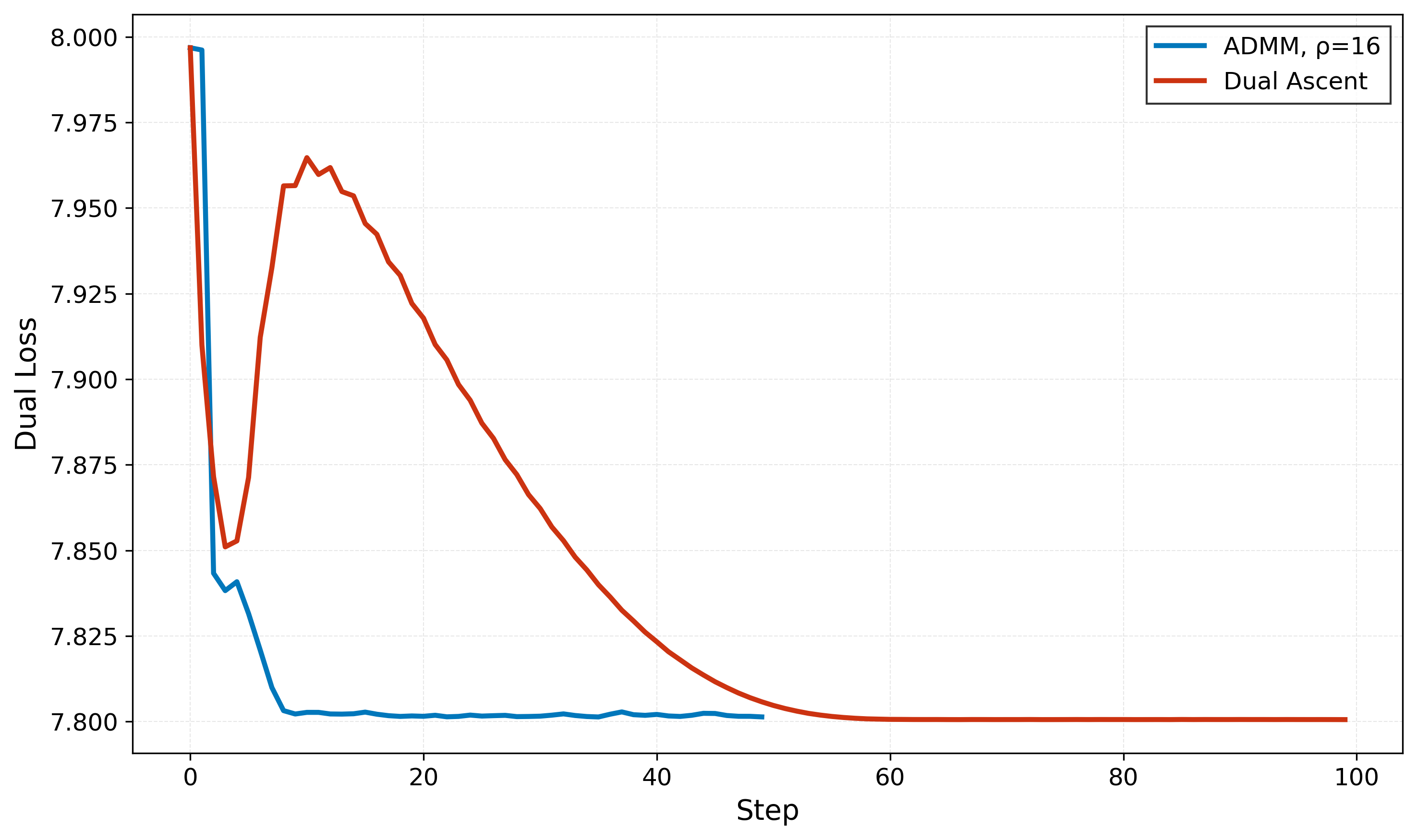
Inner Loop Convergence

We compare the inner loop losses for the best-performing hyperparameter settings above. We also compare them to dual ascent.

We can choose to visualize the inner loop loss for one of three possible weight matrices (first layer, second layer, third layer), for any one of the outer loop iterations (we do a total of five epochs over the data).

Dual ascent losses for each weight matrix in the network, for the nonzero-steps hyperparameter choices shown in the table above. Traces can be identified based on where they terminate.

Notice that both nonsmoothness and initial scale of the learning rate for dual ascent being too large both seem to play a role in the slow convergence of dual ascent in the plots above, which are evaluated for each weight matrix at the first epoch and first iteration of optimization. Dual ascent needs all 100 iterations to reach a good loss value, whereas the ADMM algorithms converge much more quickly. The ADMM algorithms only require setting the penalty parameter, and are not very sensitive to it in this experiment, as long as it is sufficiently large: we found smaller values of the penalty parameter to lead to instabilities in inner loop loss convergence, although outer loop performance was not significantly affected.¹¹

For the ADMM iteration counts, ten iterations is aggressive, but reasonable: only for fc3 does it end up a bit far from convergence, and this seems to be due to the setting of the penalty parameter we’ve chosen more than anything else.

These plots are more or less representative for all iterations of training. In later iterations, the loss decrease is often less dramatic than at the first iteration, but trends persist: dual ascent is slower, ten ADMM iterations is aggressive, but not unreasonable (see below).

Dual ascent losses for weights in the first layer of the network, for the nonzero-steps hyperparameter choices shown in the table above. Traces can be identified based on where they terminate.

Timing and Other Diagnostics

We profile the code with the pre-implemented timing commands in the original repository. It would be good to do this in a more rigorous setting, also after optimizing the code a bit more (e.g., adding compilation to unroll and fuse the inner loop where possible). But this test gives us a rough sense of how much we stand to improve.

Here are outputs for the dual ascent algorithm (100 iterations), run on a 1x H100 VM.

ubuntu@flaky-muskox-1:~/thinky-manifolds$ uv run src/main.py
Training with: manifold_muon
Epochs: 5 --- LR: 0.1
Epoch 1, Loss: 1.6895257502186054, Time: 11.8445 seconds
Epoch 2, Loss: 1.4129536565469236, Time: 11.7680 seconds
Epoch 3, Loss: 1.2799630311070656, Time: 11.7151 seconds
Epoch 4, Loss: 1.183229492635143, Time: 11.6794 seconds
Epoch 5, Loss: 1.1131725724862547, Time: 12.1164 seconds
Accuracy of the network on the 10000 test images: 52.58 %
Accuracy of the network on the 50000 train images: 65.936 %

And here are outputs for the ADMM algorithm (10 iterations).

ubuntu@flaky-muskox-1:~/thinky-manifolds$ uv run src/main.py --update manifold_muon_admm
Training with: manifold_muon_admm
Epochs: 5 --- LR: 0.1
Epoch 1, Loss: 1.6916365696459401, Time: 5.1556 seconds
Epoch 2, Loss: 1.4166164446850211, Time: 5.1545 seconds
Epoch 3, Loss: 1.2806039537702287, Time: 5.0617 seconds
Epoch 4, Loss: 1.1837433649569142, Time: 5.0579 seconds
Epoch 5, Loss: 1.1136368123852476, Time: 5.0620 seconds
Accuracy of the network on the 10000 test images: 52.62 %
Accuracy of the network on the 50000 train images: 66.086 %

We see a 2.3x speedup—not bad! We’ve cut the iteration count by a factor of 10, but ADMM uses more FLOPs per iteration because of the extra variables from splitting. With further optimizations (e.g., better fusing), it’s likely the ADMM runtime would better reflect the total iteration count and improve further.

Another natural question is the extent to which we’re obtaining ADMM iterates $(\vLambda_\star, \vX_\star)$ that satisfy the desired ADMM constraint $\vX = \vG + \vW(\vLambda + \vLambda^\top)$. We show a plot below from epoch 0, iteration 0 for the first layer (other layers/steps are similar, or better). It demonstrates that the residual norm is always rather small, but still non-negligible before convergence. Ten iterations of ADMM is not quite converged for this layer, but strikes a reasonable tradeoff between convergence and efficiency.

Feasibility ($\ell^2$ norm) for the ADMM algorithm, for the nonzero-steps hyperparameter choices shown in the table above. Traces can be identified based on where they terminate.

Conclusions

We’ve managed to speed up manifold Muon by a significant amount over the dual ascent baseline by deriving and implementing ADMM for this problem! ADMM converges faster and requires less hyperparameter tuning, allowing us to safely use a much smaller number of inner loop iterations.

You can download the code and try it yourself from my fork. I’m excited to run larger-scale experiments with this algorithm to see how it works!

As a closing thought: here’s a quote from Jeremy’s original blog post:

Manifold Muon increased the wall clock time per step compared to AdamW, although this could be improved by running fewer steps of dual ascent or adding momentum to the algorithm and running dual ascent online. Depending on other systems bottlenecks, the overhead may not be an issue.

I think the switch from dual ascent to ADMM dovetails with all of these considerations! In particular, the results on this experiment (highly clustered performance) suggest that incremental / online manifold Muon might be a natural choice for efficiency’s sake, and our ADMM algorithm should work out-of-the-box in this regime.

Cite

If you found this post or the code useful, please consider citing it:

@misc{buchanan2025mmuonadmm,
  author = {Buchanan, Sam},
  title = {Speeding Up Manifold Muon with {ADMM}},
  year = 2025,
  howpublished = {\url{https://sdbuchanan.com/blog/manifold-muon/}}
}

Postscript: Other Quadratic Constraints

Another recent blog post by Ben Keigwin, Dhruv Pai, and Nathan Chen at Tilde Research describes how the essential structure of the manifold Muon algorithm is preserved under replacements of the constraint $\vW^\top \vW = \vI$ by similar constraints (e.g., constraining only the diagonal) (Keigwin et al., 2025). As a corollary, the ADMM algorithm we derived above can be applied to constraints from this family with little extra effort! We leave this as an exercise to the reader.

Acknowledgments

Thanks to Jeremy Bernstein for helpful discussions. Thanks to the TRC program, Hyperbolic, and Mithril for compute.

1. Here and below, we write $\ip{\vA}{\vB} = \tr(\vA^\top \vB) = \sum_{i, j} A_{ij} B_{ij}$ to denote the Frobenius inner product on matrices, which treats them as if they were vectors, and $\norm{\spcdot}$ to denote the operator norm (or spectral norm, or Schatten $\infty$-norm), which is the largest singular value of its (matrix) argument. ↩

2. As written, the matrix sign function is only defined for inputs that have no zero singular values. It turns out that as long as $\vA$ satisfies the tangent constraint $ \vA^\top \vW + \vW^\top \vA = \Zero$, the update $\vW -\eta \vA$ never has zero singular values! This can be derived straightforwardly via contradiction, and provides a strong motivation for the need to exactly solve the manifold Muon subproblem. ↩

3. Here and below, we write $\norm{\spcdot}_*$ to denote the nuclear norm (or Schatten 1-norm), which is the sum of the singular values of its (matrix) argument. ↩

4. Less naive algorithms for nonsmooth optimization can ameliorate this pathological behavior, sometimes to a significant extent. See, for example, work of Damek Davis and collaborators (Davis et al., 2024). These algorithms definitely merit a closer look in the context of manifold Muon! But we will stick our neck out and suggest that it might be hard to beat ADMM’s solution quality vs. iteration count tradeoff, based on the experiments to come—although we would be happy to be proven wrong. ↩

5. We’ll see this is indeed the case empirically in our experiments below! ↩

6. This is a relatively straightforward argument, but at the same time, I haven’t seen it anywhere in the compressed sensing literature previously (and this literature applied singular value thresholding to almost everything one could). If you know of a reference that has applied this previously, please let me know! ↩

7. After writing down these updates all together, it becomes clear that $\vLambda_{k+1}$ is always a symmetric matrix. We use this invariant to simplify some steps in the algorithm here and below! ↩

8. More precisely, it’s straightforward to prove (using the SVD) that singular value thresholding is a $1$-Lipschitz continuous function of the input matrix with respect to the operator norm. ↩

9. It may be obvious, but it’s worth repeating: the Manifold Muon runs an iterative optimization solver after every forward/backward pass of the model being trained, for every weight matrix in the model. This leads to some interesting debugging issues, such as small differences in the final solution obtained by different manifold Muon solvers at iteration zero leading to significant differences in the behavior of subsequent gradients/inner loop solves (even though everything is convex!). These differences seem to mostly be restricted to inner loop loss, as final val error does not seem to very much, but it will be interesting to study this behavior at larger scales. ↩

10. For the sake of comparison, we also use this initialization for our $\vLambda$ in our ADMM algorithm. ↩

11. This is likely because of the fact that we compute msign with an approximate algorithm, leading to unstable behavior when we aggressively threshold singular values in the $\vX$ update of ADMM. ↩

References

- (2025). The Polar Express: Optimal matrix sign methods and their application to the Muon algorithm. arXiv [cs.LG].
- (2025). Steepest Descent on Finsler-Structured (Matrix) Manifolds. Retrieved from https://leloykun.github.io/ponder/steepest-descent-finsler/
- (2024). Stochastic algorithms with geometric step decay converge linearly on sharp functions. Mathematical programming, 207(1-2), 145–190.
- (2022). High-Dimensional Data Analysis with Low-Dimensional Models: Principles, Computation, and Applications. Cambridge University Press, 2022.
- (2015). Adaptive Primal-Dual Splitting Methods for Statistical Learning and Image Processing. In Advances in Neural Information Processing Systems. Curran Associates, Inc..
- (2011). Distributed Optimization and Statistical Learning via the Alternating Direction Method of Multipliers. Foundations and Trends® in Machine Learning, 3(1), 1–122.